Using Simulations to Check Your Statistical Intuition

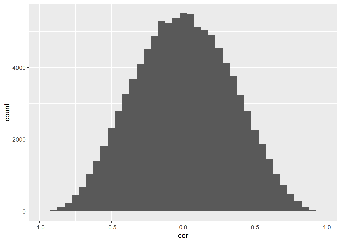
R’s distribution simulation functions (e.g. dbinom, runif) make it quick and easy to double check one’s intuitions. For example, I’d been thinking that under H0 the distribution of correlations from normal samples should drop off sharply as you go away from 0 such that a shift in correlation from 0 -> 0.1 is much more likely than 0.8 -> 0.9.

So I used purrr::map() to run a quick simulation. Here we simulate the null distribution based on 100,000 observations and compute the chance of a value being above 0.7. If it was uniform we would expect ~15% (.03/2) of the distribution to be here but end up with ~1.2% with the drop off.

library(tidyverse)

── Attaching core tidyverse packages ──────────────────────── tidyverse 2.0.0 ──
✔ dplyr     1.1.4     ✔ readr     2.1.5
✔ forcats   1.0.0     ✔ stringr   1.5.1
✔ ggplot2   3.5.0     ✔ tibble    3.2.1
✔ lubridate 1.9.3     ✔ tidyr     1.3.1
✔ purrr     1.0.2     
── Conflicts ────────────────────────────────────────── tidyverse_conflicts() ──
✖ dplyr::filter() masks stats::filter()
✖ dplyr::lag()    masks stats::lag()
ℹ Use the conflicted package (<http://conflicted.r-lib.org/>) to force all conflicts to become errors

set.seed(89745) 
cor_check <- map(1:100000, function(i){ 
  cor(rnorm(10), rnorm(10), method = "pearson") 
}) 
cor_check <- data.frame(cor = do.call(rbind, cor_check))

mean(cor_check$cor >= 0.7)*100 

[1] 1.227

#1.227 Percent 

ggplot(cor_check, aes(x = cor))+
  geom_histogram(binwidth = 0.05)