Simulation as a Super Power

Writing simulations is one of the best ways I’m aware of to build one’s statistical intuition and comfort with data visualization. In addition to being able to try out new statistical tests and know exactly what effects they should find, they’re also great for communicating ideas and persuading others.

A few months ago I had occasion to do just that.

\[...\]

At the time I was advocating in a manuscript that when one needs to make a prediction combining predictions from different models is the way to go. Specifically, my results suggest that using a weighted average to make accurate models more influential. To do this, the predictions from each model are multiplied by the inverse of the model’s root mean squared error (rmse) of the model and summed. Someone helping me improve this manuscript thought that instead I should be weighting by the inverse of the model’s variance. This is a reasonable expectation (variance weighting is beautifully explained here) so I needed to convince my collaborator before the manuscript was ready for the world – Here’s how I did this with in a simulation that was only about 100 lines¹ of R code.

Simulating Observations

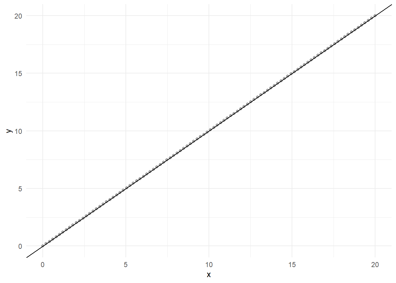
Let’s imagine we’re studying dead simple system where the output is equal to the input (\(y = 0 + 1*x\)). We can simulate as many samples as we would like from this system over a range of xs.

n = 100 # samples to be generated
xs <- seq(0, 20, length.out = n) # x values evenly spaced from 0-20 
ys <- 0+1*xs

Here’s the simulated “data”.

Now we can simulate models that are trying to predict y. To do this we’ll think of a model as being equivalent to the true value of y plus some model specific error. If we assume that the models aren’t prone to systematically over or underestimating, then we can use a normal distribution to generate these errors like so:

mean1 =  0 # error doesn't tend to be over or under
var1  =  1 # variance of the error
y1 <- ys + rnorm(n = n, mean = mean1, sd = sqrt(var1))

We can simulate a better model by decreasing the variance (errors are consistently closer to the mean of 0). Conversely we can simulate a worse model by making the model tend to over or undershoot by changing the mean or make larger errors more common by increasing the varience. Here’s a model that’s worse than the previous one.

mean2 =  1 # predictions tend to overshoot
var2  = 10 # larger errors are more common
y2 <- ys + rnorm(n = n, mean = mean2, sd = sqrt(var2))

Let’s look at the predictions from model y1 and model y.

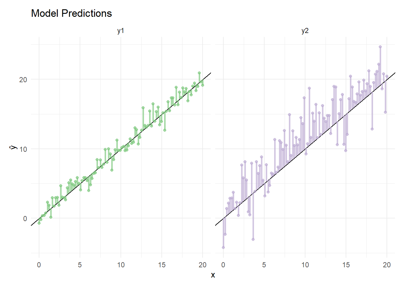
Here we can see that y1’s error (vertical lines) are considerably smaller than that of y2.

We can subtract the true value \(y\) from the predicted value \(\hat y\) to see this more clearly.

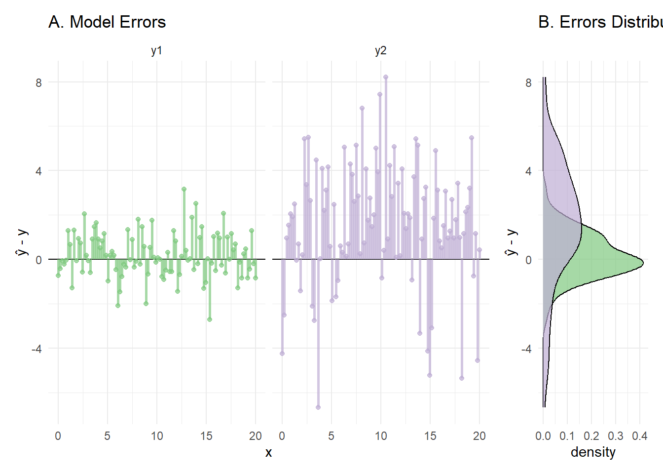
In panel B we can see the difference between the two error distributions for the models (save a few irregularities in these distributions from only using 100 samples.

Now we can try out different averaging schemes to cancel out some of the error and get a better prediction. We can test a simple average like so.

e1 <- 0.5*y1 + 0.5*y2

We can also try placing more weight on models with less variable predictions (and hopefully smaller errors).

yhat_vars  <- unlist(map(list(y1, y2), function(e){var(e)})) # Calculate variance for each model's predictions
wght_vars  <- (1/yhat_vars)/sum(1/yhat_vars) # Take the inverse and get percent weight by dividing by the sum 
e2 <- wght_vars[1]*y1  + wght_vars[2]*y2 # Scale each model's prediction and add to get the weighted average.

We can also try placing more weigh on models that are more accurate².

yhat_rmses <- unlist(map(list(y1, y2), function(e){sqrt((sum((ys-e)**2)/n))}))
wght_rmses <- (1/yhat_rmses)/sum(1/yhat_rmses)
e3 <- wght_rmses[1]*y1 + wght_rmses[2]*y2

Now we can calculate the RMSE for both models and these weighed averages.

name	y_rmse	mean1	mean2	var1	var2
y1	1.023765	0	1	1	10
y2	3.218318	0	1	1	10
unif	1.796390	0	1	1	10
var	1.670037	0	1	1	10
rmse	1.217204	0	1	1	10

y1 is the best set of predictions, averaging did not benefit predicitons here. This is not too much of a shock since y2 was generated by a model that was prone to systematically overshooting the true value and was more likely to have bigger errors.

But how would these results change if the models were more similar? What if the models had more similar error variences? Or if one was prone to overshooting while the other was prone to undershooting?

Expanding the Simulation

To answer this we can package all the code above into a function with variables for each models’ error distribution and how many observations to simulate and return the RMSE for each model. This function (run_sim) is a little lengthy so I’ve collapsed it here:

run_sim <- function(
    n = 10000,
    mean1 = 0,
    mean2 = 1, 
    var1 = 1,
    var2 = 10
  ){
  xs <- seq(0, 20, length.out = n)
  ys <- 0+1*xs

  # Simulate models
  y1 <- ys + rnorm(n = n, mean = mean1, sd = sqrt(var1))
  y2 <- ys + rnorm(n = n, mean = mean2, sd = sqrt(var2))
  
  # Equal weights
  e1 <- 0.5*y1 + 0.5*y2
  
  # Variance weights
  yhat_vars  <- unlist(map(list(y1, y2), function(e){var(e)}))
  wght_vars  <- (1/yhat_vars)/sum(1/yhat_vars)
  e2 <- wght_vars[1]*y1 + wght_vars[2]*y2
  
  # RMSE weights
  yhat_rmses <- unlist(map(list(y1, y2), function(e){sqrt((sum((ys-e)**2)/n))}))
  wght_rmses <- (1/yhat_rmses)/sum(1/yhat_rmses)
  e3 <- wght_rmses[1]*y1 + wght_rmses[2]*y2
  
  # Aggregate predictions and accuracy
  data <- data.frame(xs, ys, y1, y2, unif = e1, var = e2, rmse = e3)
  plt_data <- data %>% 
    select(-xs) %>% 
    pivot_longer(cols = c(y1, y2, unif, var, rmse)) %>% 
    rename(y_pred = value) %>% 
    # Calc RMSE
    group_by(name) %>%                
    mutate(y_se = (ys - y_pred)**2) %>% 
    summarise(y_rmse = sqrt(mean(y_se))) %>% 
    ungroup() %>% 
    mutate(mean1 = mean1,
           mean2 = mean2,
           var1 = var1,
           var2 = var2)
  
  return(plt_data)
}

Next we’ll define the variables to examine in our computational experiment.

We can think about combining models that differ in accuracy (error mean) and precision (error variation). These differences can be are easier to think about visually. Here are the four “flavors” of model that we would like to combine to test all combinations of accuracy and precision.

Warning: Using `size` aesthetic for lines was deprecated in ggplot2 3.4.0.
ℹ Please use `linewidth` instead.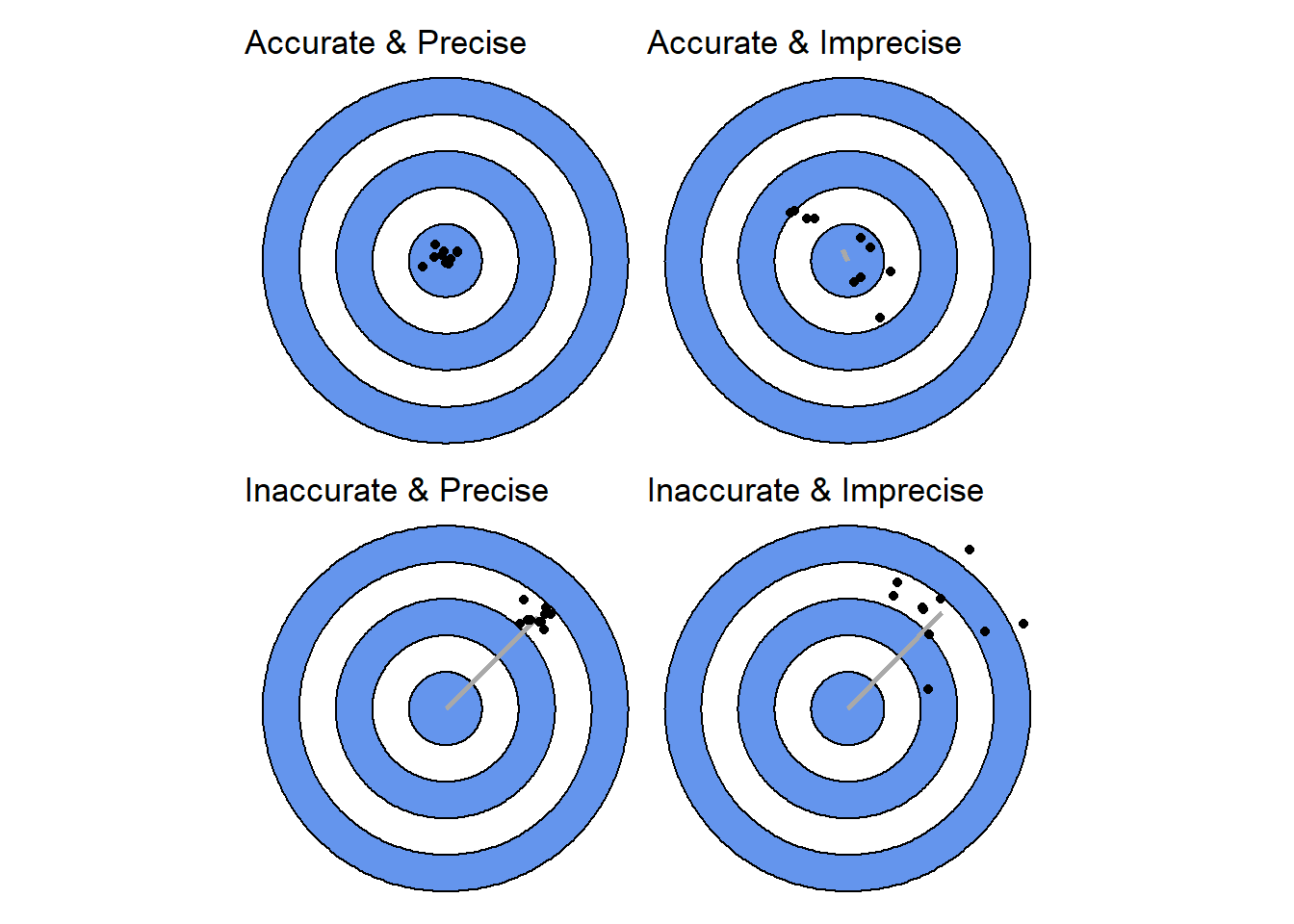

Specifically, We’ll have one model that acting as a stable reference and vary the error of the other (y2). We’ll make a version of the y2 model that is accurate (the mean error is only shifted by 0.01) and one that is inaccurate (the mean error is shifted by 50). Then we’ll see what happens when these two go from being precise (variance around 0.01) to very imprecise (variance up to 100).

In R this is expressed as below. When the mean of the error (mean_shift) is near zero accuracy is high. When the variance of the error (var_shift) is near zero precision is high.

params <- expand.grid(
  mean_shift = seq(0.01, 50, length.out = 2),
  var_shift = c(seq(0.01, 0.99, length.out = 50), seq(1, 100, length.out = 90))
)

This results in quite a few (280) combinations. of parameters Let’s look at the first and last few:

	mean_shift	var_shift
1	0.01	0.01000
2	50.00	0.01000
3	0.01	0.03000
278	50.00	98.88764
279	0.01	100.00000
280	50.00	100.00000

Now we’ll generate the results. This code may look confusing at first. Here’s what it’s doing. 1. run_sim executes the steps we did above, using the parameters we specified in params to generate 100,000 observations and calculate the expected RMSE of each approach. 1. map is a way of looping over some input and putting all of the results into a list. In this case we’re looping over all the the rows in params so we will end up with a list containing a data.frame for each of the 280 parameter combinations. 1. rbind will combine two data.frames, ‘stacking’ one on top of the other. However, it can’t use a list as input so… 1. we have to use do.call. It will iteratively apply a function (rbind) to the entries in a list so that all the simulation results end up in one big data.frame.

sim_data <- do.call(         # 4.
  rbind,                     # 3
  map(seq(1, nrow(params)),  # 2.
      function(i){           
        run_sim(             # 1.
          n = 10000,
          mean1 = 0,
          mean2 = unlist(params[i, 'mean_shift']), 
          var1 = 1,
          var2 = unlist(params[i, 'var_shift']))
      })
)

Once this runs we can look at the results. Let’s consider the high accuracy y2 first, starting where y2’s variance is less than or equal to y1’s variance (1).

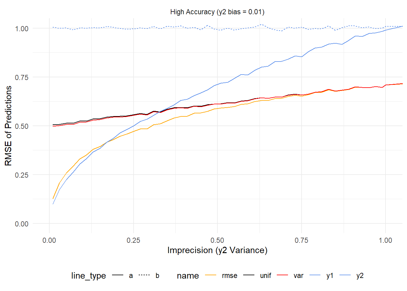
When y2’s variance is very small (< ~0.2) it outperforms all other estimates (just like the previous simulation). As it increases it crosses the line for \(rmse^{-1}\) weighting (rmse, orange line) and then the other averaging schemes before converging with y1 (dashed blue line). Over the same span \(rmse^{-1}\) converges with \(var^{-1}\) (var, red line), and the simple average (unif, black line).

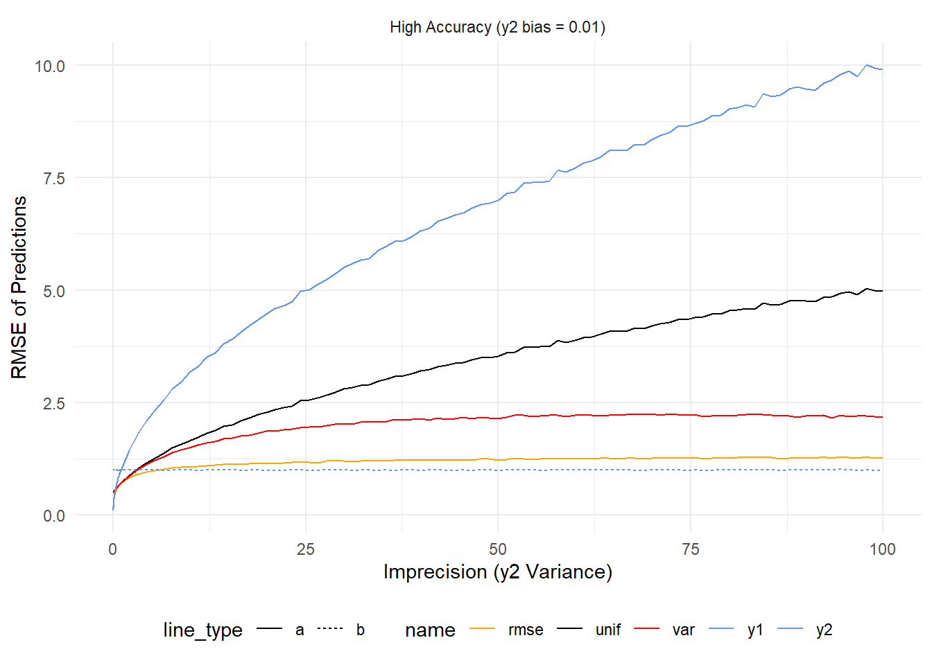
As y2 continues to worsen, every prediction (except those from y1) get worse and worse. What’s interesting is that this doesn’t happen at the same rate. Because \(rmse^{-1}\) weighting penalizes predictions from models based on accuracy its error grows much more slowly than \(var^{-1}\) weighting or uniform weighting.

To summarize – If two models are equally good (1 on the y axis) then using any of the averaging strategies here will be better than not averaging. If one is far and away better than the other then it’s best to ignore the worse one. In practice one might find they have models that are performing in the same ballpark of accuracy. These results would suggest that in that case one gets the best results by \(rmse^{-1}\) weighting.

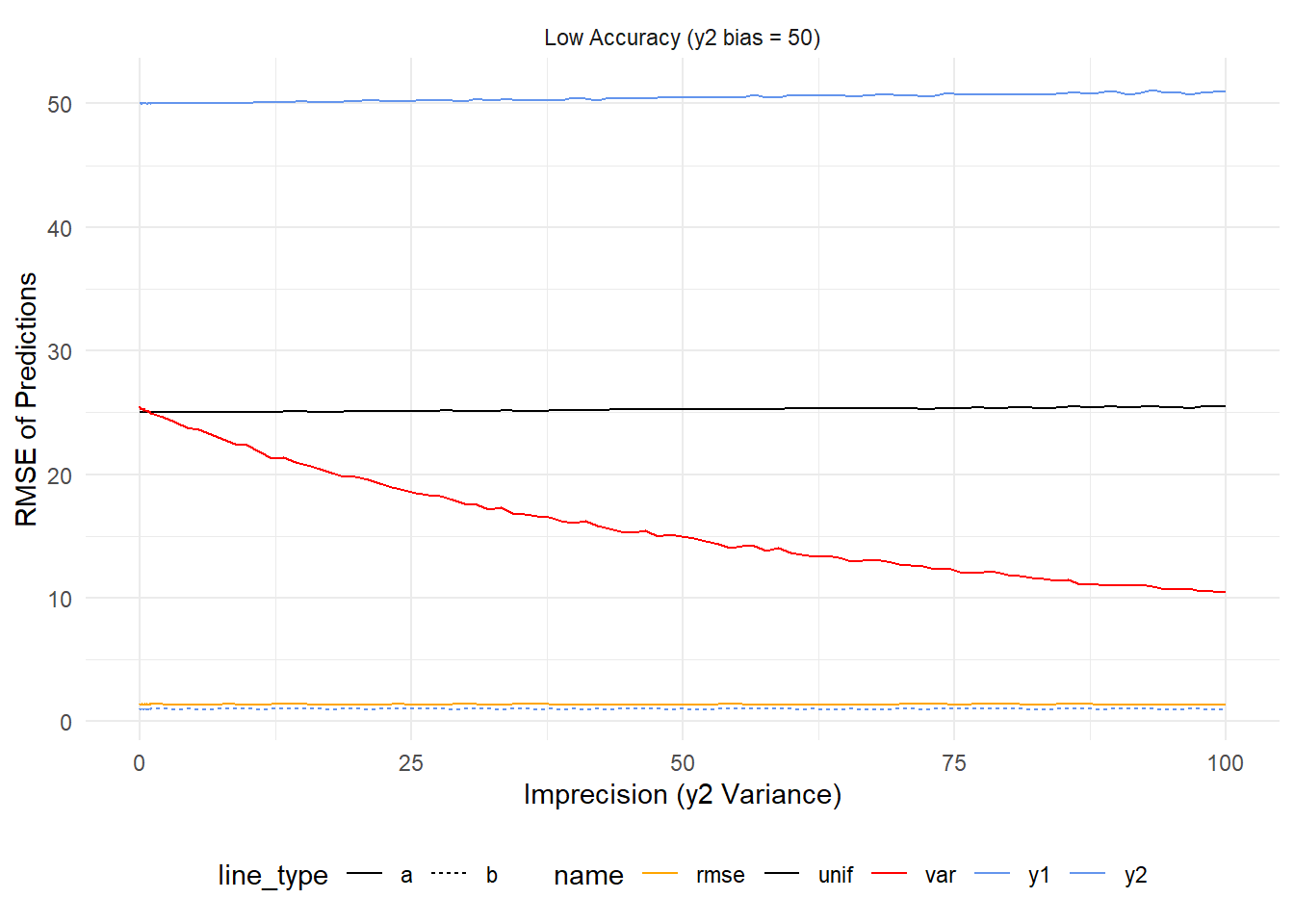
Now let’s add in the case where one model is highly inaccurate. In this case, as precision worsens y2 (top blue line) has higher error but this is hard to see given just how much error it has to begin with. Uniform weighting follows a similar trend (but lessened by half) while \(var^{-1}\) improves as y2 becomes more imprecise because this decreases it’s influence on the final prediction. Of the averages \(rmse^{-1}\) is the best by a country mile because it accounts for the inaccuracy of y2 right from the start.

What if models err in different directions?

Just for fun, let’s add one more simulation. Let’s suppose we have two models that are equally precise but err in opposite directions. We can modify the code above like so to have some combinations that are equally accurate (just in oppostie directions) and with differing accuracies.

shift_array = seq(0.01, 10, length.out = 40)
params <- expand.grid(
  mean_shift  =    shift_array,
  mean_shift2 = -1*shift_array
)

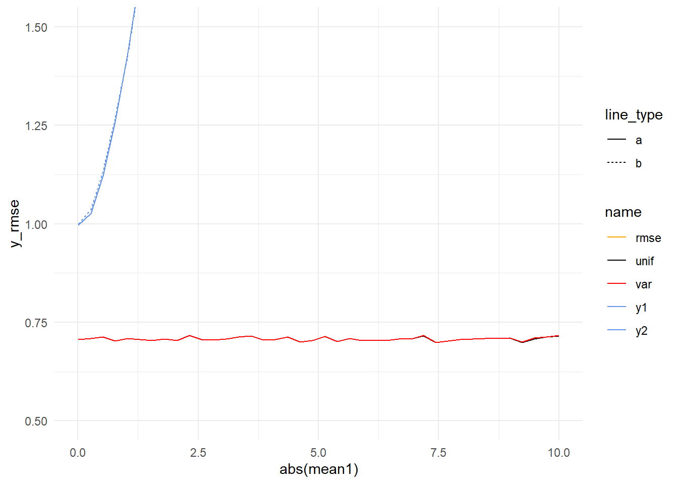
Let’s consider the case where errors are equal and opposite. In the previous simulation, when model variances were equal (1) the performance of all the averages converged, so we might expect that to be the case here. We can see the models getting worse and worse, but can’t see what’s happening with the averages.

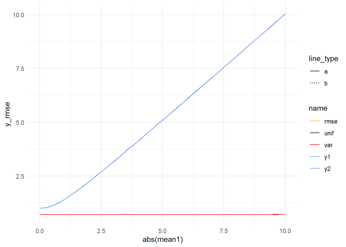
If we zoom in, it looks like our intuition is correct (ignoring some sampling noise).

But we also simulated combinations where one model was off by more than the other. Let’s plot all the combinations of mean1 and mean2 but instead of showing the error of each method like we’ve done above, let’s instead just show where each method produces the best results.

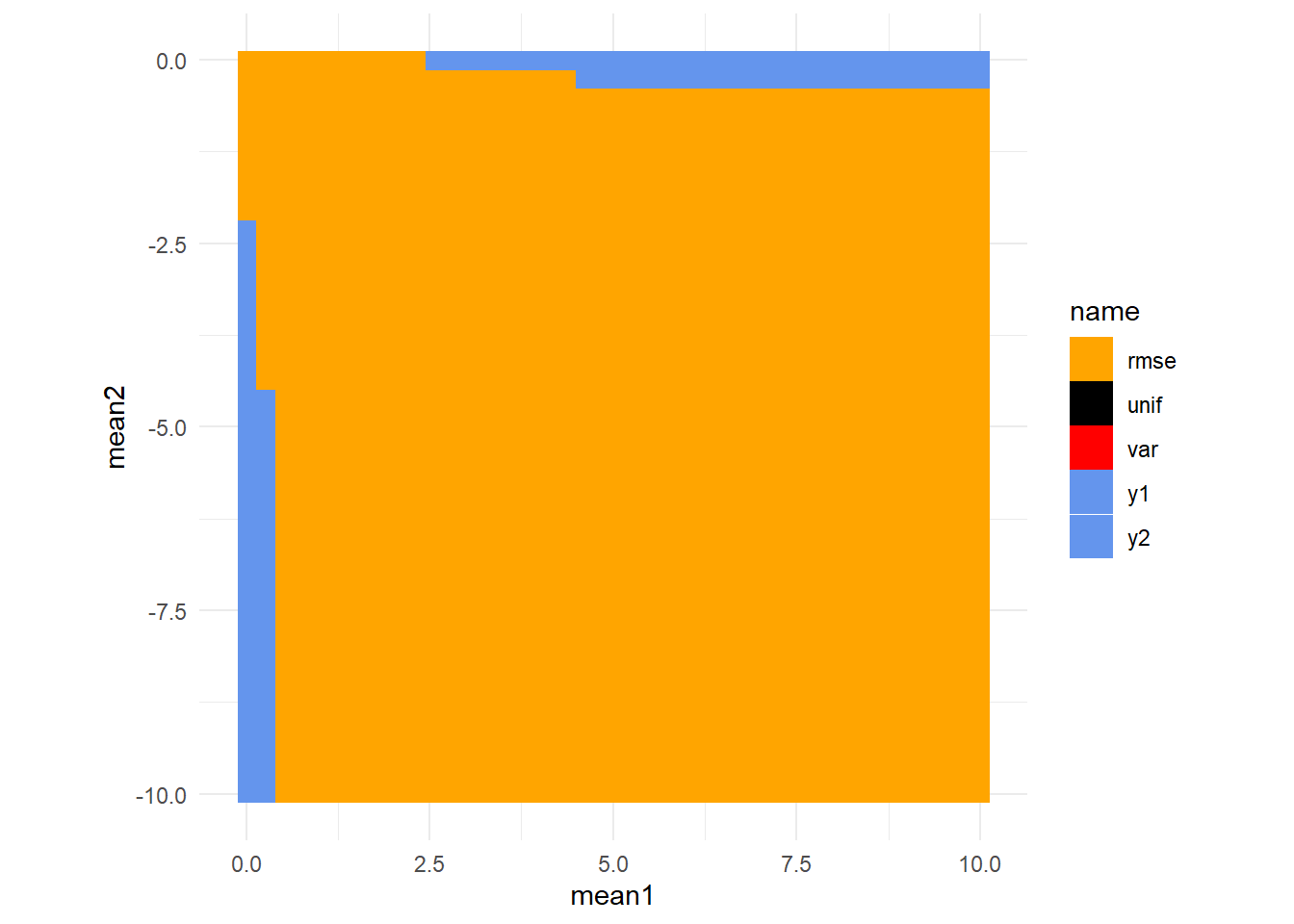
Consistent with what we’ve seen, for most of these combinations \(rmse^{-1}\) performs best. We can get a little fancier by color coding each fo these cells by the best expected error (y_rmse) and color coding the border with the method that produced the best expected error (excepting \(rmse^{-1}\) since that accounts for so much of the space).

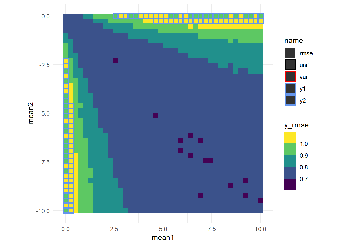
It looks like there’s a sort of saddle shape off the diagonal. We’ll re-plot these data in 3d so we can usethe z axis for y_RMSE and color code each point as above.

There we go. Just a little bit of scripting and plotting will let one answer a whole lot of questions about statistics.

Footnotes

1. I added a fair bit more for the sake of this post

2. For simplicity we’re not using testing and training sets. In this simulation that shouldn’t be an issue, but one might consider cases where this could matter. For instance if one model was wildly over fit then its RMSE would not be predictive of its RMSE on newly collected data